ItwasWritten

Real-Time Artistry: Deconstructing Fast Neural Style Transfer

Stylized Example

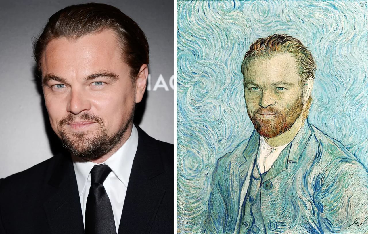
Ever wished you could instantly repaint your photos in the style of a masterpiece of Picasso, Monet or VanGogh ? This is the promise of Neural Style Transfer (NST), a deep learning technique that recombines the content of one image with the style of another.

It was introduced firstly in Gatys.et.al 2015 paper, however,it was incredibly slow. It optimized each new image pixel by pixel, a process taking minutes or hours, which made real-time applications like video filters impossible.

This limitation was overcomed by Johnson.et.al 2016 paper that led to the development of Fast Neural Style Transfer. Instead of optimizing an image, this approach trained a dedicated neural network once for a specific style, generating the art much faster.

In this blog, I would dive into the mechanics behind the Johnson.et.al paper. We'll deconstruct the elegant two-network architecture, explore the clever loss functions that mathematically define "content" and "style," and walk through the training process that brings it all together. Let's get started!

What We'll Cover

Before we dive into the nuts and bolts of Fast Neural Style Transfer, let’s take a step back and outline the journey we’re about to take. Think of this as a roadmap: by the time you’ve reached the end, you’ll understand not only the what but also the why of each component.

We’ll begin with the architecture itself. Fast Neural Style Transfer relies on two very different networks working hand in hand. The first is the Image Transformation Network, which is the actual model we train. You can think of it as the artist — it takes a content image as input and produces a stylized version as output. The second is the Loss Network, which plays the role of an art critic. Instead of being trained from scratch, this one is a pre-trained model (VGG-16) that we borrow to evaluate how well the artist has captured both the content of the photo and the style of the artwork.

Once we understand these two roles — the artist and the critic — we’ll move on to the loss functions that define how we measure success. These are the rules of the game. We’ll see how the network is guided to keep the structure of the original image intact (content loss), while also absorbing the textures, brushstrokes, and color palettes of the chosen style image (style loss). Alongside these, we’ll also introduce a smoothing term (total variation loss) to ensure the final output looks natural and visually pleasing.

In short, this blog will cover three main pillars: the two-network architecture, the language of loss functions, and the training loop that makes it all work.

The Architecture: Team of Two Networks

At the heart of Fast Neural Style Transfer lies working of two different kinds of neural networks. One of them is the Image Transformation Network, the model we actually train. It is the artist — the one who takes in an ordinary photo and repaints it in the style of a chosen artwork. The other is the Loss Network, a pre-trained VGG model, which plays the role of the art critic. The critic doesn’t paint anything itself, but it evaluates the artist’s work and provides the feedback necessary for learning.

A. The Image Transformation Network (The "Artist")

This is the model we actually train. Its job is straightforward: take a normal photo (the content image) and instantly produce a new version that looks like it was painted in the style of an artwork. Think of it as an artist who has practiced one style so much that they can apply it to any new scene in seconds.

import torch

class TransformerNet(torch.nn.Module):
    def __init__(self):
        super().__init__()
        # Non-linearity
        self.relu = torch.nn.ReLU()

        # Down-sampling convolution layers
        num_of_channels = [3, 32, 64, 128]
        kernel_sizes = [9, 3, 3]
        stride_sizes = [1, 2, 2]
        self.conv1 = ConvLayer(num_of_channels[0], num_of_channels[1], kernel_size=kernel_sizes[0], stride=stride_sizes[0])
        self.in1 = torch.nn.InstanceNorm2d(num_of_channels[1], affine=True)
        self.conv2 = ConvLayer(num_of_channels[1], num_of_channels[2], kernel_size=kernel_sizes[1], stride=stride_sizes[1])
        self.in2 = torch.nn.InstanceNorm2d(num_of_channels[2], affine=True)
        self.conv3 = ConvLayer(num_of_channels[2], num_of_channels[3], kernel_size=kernel_sizes[2], stride=stride_sizes[2])
        self.in3 = torch.nn.InstanceNorm2d(num_of_channels[3], affine=True)

        # Residual layers
        res_block_num_of_filters = 128
        self.res1 = ResidualBlock(res_block_num_of_filters)
        self.res2 = ResidualBlock(res_block_num_of_filters)
        self.res3 = ResidualBlock(res_block_num_of_filters)
        self.res4 = ResidualBlock(res_block_num_of_filters)
        self.res5 = ResidualBlock(res_block_num_of_filters)

        # Up-sampling convolution layers
        num_of_channels.reverse()
        kernel_sizes.reverse()
        stride_sizes.reverse()
        self.up1 = UpsampleConvLayer(num_of_channels[0], num_of_channels[1], kernel_size=kernel_sizes[0], stride=stride_sizes[0])
        self.in4 = torch.nn.InstanceNorm2d(num_of_channels[1], affine=True)
        self.up2 = UpsampleConvLayer(num_of_channels[1], num_of_channels[2], kernel_size=kernel_sizes[1], stride=stride_sizes[1])
        self.in5 = torch.nn.InstanceNorm2d(num_of_channels[2], affine=True)
        self.up3 = ConvLayer(num_of_channels[2], num_of_channels[3], kernel_size=kernel_sizes[2], stride=stride_sizes[2])

    def forward(self, x):
        y = self.relu(self.in1(self.conv1(x)))
        y = self.relu(self.in2(self.conv2(y)))
        y = self.relu(self.in3(self.conv3(y)))
        y = self.res1(y)
        y = self.res2(y)
        y = self.res3(y)
        y = self.res4(y)
        y = self.res5(y)
        y = self.relu(self.in4(self.up1(y)))
        y = self.relu(self.in5(self.up2(y)))


class ConvLayer(torch.nn.Module):
    def __init__(self, in_channels, out_channels, kernel_size, stride):
        super().__init__()
        self.conv2d = torch.nn.Conv2d(in_channels, out_channels, kernel_size, stride, padding=kernel_size//2, padding_mode='reflect')

    def forward(self, x):
        return self.conv2d(x)


class ResidualBlock(torch.nn.Module):

    def __init__(self, channels):
        super(ResidualBlock, self).__init__()
        kernel_size = 3
        stride_size = 1
        self.conv1 = ConvLayer(channels, channels, kernel_size=kernel_size, stride=stride_size)
        self.in1 = torch.nn.InstanceNorm2d(channels, affine=True)
        self.conv2 = ConvLayer(channels, channels, kernel_size=kernel_size, stride=stride_size)
        self.in2 = torch.nn.InstanceNorm2d(channels, affine=True)
        self.relu = torch.nn.ReLU()

    def forward(self, x):
        residual = x
        out = self.relu(self.in1(self.conv1(x)))
        out = self.in2(self.conv2(out))
        return out + residual  # modification: no ReLu after the addition


class UpsampleConvLayer(torch.nn.Module):

    def __init__(self, in_channels, out_channels, kernel_size, stride):
        super().__init__()
        self.upsampling_factor = stride
        self.conv2d = ConvLayer(in_channels, out_channels, kernel_size, stride=1)

    def forward(self, x):
        if self.upsampling_factor > 1:
            x = torch.nn.functional.interpolate(x, scale_factor=self.upsampling_factor, mode='nearest')
        return self.conv2d(x)

How it works:

Down-sampling (Seeing the big picture): The first few convolutional layers reduce the resolution of the image while increasing the number of feature channels. This is like zooming out — the network focuses on the overall structure of the image instead of pixel-level details. It captures shapes, outlines, and object placement.
Residual Blocks (Adding style without losing content): At the core, the image passes through several residual blocks. These blocks apply transformations while keeping a shortcut connection to the original input. In simple terms, the block says: “Keep what’s already important, but add some stylistic flair on top.” This ensures the main content of the photo isn’t lost, while brushstrokes and textures are layered in.
Up-sampling (Bringing back the details): After processing, the image needs to be expanded back to its original size. Instead of transposed convolutions (which often create ugly checkerboard artifacts), the network uses a cleaner approach: nearest-neighbor up-sampling followed by a convolution. This produces smoother, artifact-free images — closer to how an artist fills in fine details after rough sketches.
Instance Normalization (The secret sauce): A subtle but crucial detail is the use of Instance Normalization instead of Batch Normalization. While BatchNorm normalizes across a whole batch of images, InstanceNorm works on each image individually. This matters because style is highly image-specific — one photo may be bright, another dark, and forcing them into a batch average often dulls the effect. InstanceNorm ensures the style is applied cleanly and consistently to each image.

The result is a lightweight artist that can instantly repaint any photo in the trained style.

B. The Loss Network (The "Art Critic")

Now, an artist needs feedback. That’s where the Loss Network comes in — the art critic that judges the quality of the stylized image.

Here’s the trick: instead of training the artist by comparing pixel-by-pixel differences (which would make the output blurry), we use a pretrained CNN (often VGG-16) as a critic. This network isn’t trained during our process — it’s frozen — but its feature maps provide the vocabulary to measure style and content.

from collections import namedtuple
import torch
from torchvision import models

class Vgg16(torch.nn.Module):
    def __init__(self, requires_grad=False, show_progress=False):
        super().__init__()
        vgg16 = models.vgg16(pretrained=True, progress=show_progress).eval()
        vgg_pretrained_features = vgg16.features
        self.layer_names = ['relu1_2', 'relu2_2', 'relu3_3', 'relu4_3']
        self.slice1 = torch.nn.Sequential()
        self.slice2 = torch.nn.Sequential()
        self.slice3 = torch.nn.Sequential()
        self.slice4 = torch.nn.Sequential()
        for x in range(4):
            self.slice1.add_module(str(x), vgg_pretrained_features[x])
        for x in range(4, 9):
            self.slice2.add_module(str(x), vgg_pretrained_features[x])
        for x in range(9, 16):
            self.slice3.add_module(str(x), vgg_pretrained_features[x])
        for x in range(16, 23):
            self.slice4.add_module(str(x), vgg_pretrained_features[x])

        if not requires_grad:
            for param in self.parameters():
                param.requires_grad = False

    def forward(self, x):
        x = self.slice1(x)
        relu1_2 = x
        x = self.slice2(x)
        relu2_2 = x
        x = self.slice3(x)
        relu3_3 = x
        x = self.slice4(x)
        relu4_3 = x
        vgg_outputs = namedtuple("VggOutputs", self.layer_names)
        out = vgg_outputs(relu1_2, relu2_2, relu3_3, relu4_3)
        return out

# Set the perceptual loss network to be VGG16
PerceptualLossNet = Vgg16

How the critic evaluates:

Content Loss: The critic looks at certain higher-level layers of VGG (like relu3_3) to check if the main objects and structure of the stylized image still match the original content image. Mathematically, it’s the mean squared error between feature representations:

L_{content}(\hat{y}, y_c) = \| F^l(\hat{y}) - F^l(y_c) \|^2

where $F^l(x)$ is the feature map of image $x$ at layer $l$ .

Style Loss: To check if the style matches, the critic compares the correlations between feature maps using Gram matrices. This captures textures and patterns rather than exact pixels:

L_{style}(\hat{y}, y_s) = \sum_l \| G^l(\hat{y}) - G^l(y_s) \|^2

where $G^l(x) = F^l(x) F^l(x)^T$ is the Gram matrix of features at layer $l$ .

Total Variation Loss: Finally, to keep the image smooth and natural (no noisy patches), we add a regularization term called total variation loss:

L_{tv}(\hat{y}) = \sum_{i,j} ( (\hat{y}_{i,j+1} - \hat{y}_{i,j})^2 + (\hat{y}_{i+1,j} - \hat{y}_{i,j})^2 )

Final Judgment:

The overall loss is a weighted sum:

L = \alpha L_{content} + \beta L_{style} + \gamma L_{tv}

Here, $\alpha, \beta, \gamma$ control how much importance we give to content preservation, style matching, and smoothness.

In short, the artist generates stylized images, while the critic ensures they stay true to the content and faithfully adopt the chosen style. Together, they create art.

The Training Loop – Bringing It All Together

Now that we have our artist (Image Transformation Network) and critic (Loss Network), it’s time to teach the artist how to paint. The training loop is essentially an iterative learning process where the artist tries, the critic evaluates, and the artist improves.

import os
import time
import torch
from torch.optim import Adam
import numpy as np
import cv2 as cv

TRAINING_CONFIG = {
    "dataset_path": "./data/mscoco",
    "style_image_path": "./data/style-images/starry_night.jpg",
    "output_model_dir": "./models/binaries",

    # --- Training Hyperparameters ---
    "image_size": 256,
    "batch_size": 4,
    "num_of_epochs": 2,
    "subset_size": 20000, # Use a subset of the dataset for faster training example

    # --- Loss Weights ---
    "content_weight": 1e0,  # Corresponds to alpha
    "style_weight": 4e5,   # Corresponds to beta
    "tv_weight": 1e-6,     # Total Variation loss weight for regularization

    # --- Logging ---
    "log_freq": 500, # Print loss every 500 batches
}


def train(config):
    # Set the device (GPU if available, otherwise CPU)
    device = torch.device("cuda" if torch.cuda.is_available() else "cpu")
    print(f"Using device: {device}")

    train_loader = utils.get_training_data_loader(config)


    perceptual_loss_net = PerceptualLossNet(requires_grad=False).to(device)


    optimizer = Adam(transformer_net.parameters())

    style_img = utils.prepare_img(config['style_image_path'], target_shape=None, device=device, batch_size=config['batch_size'])
    style_img_feature_maps = perceptual_loss_net(style_img)
    target_style_grams = [utils.gram_matrix(x) for x in style_img_feature_maps]

    print("--- Starting Training ---")
    ts = time.time()

    # 5. Start Training Loop
    for epoch in range(config['num_of_epochs']):
        for batch_id, (content_batch, _) in enumerate(train_loader):
            # Move the content batch to the correct device
            content_batch = content_batch.to(device)

            # --- Forward Pass ---
            # Generate a stylized image by passing the content image through the transformer network
            stylized_batch = transformer_net(content_batch)

            # --- Loss Calculation ---
            # Get feature maps for both the original content and the stylized image
            content_feature_maps = perceptual_loss_net(content_batch)
            stylized_feature_maps = perceptual_loss_net(stylized_batch)

            # a) Content Loss
            # We want the feature representation of the stylized image to be similar
            # to the feature representation of the original content image.
            target_content_repr = content_feature_maps.relu2_2
            current_content_repr = stylized_feature_maps.relu2_2
            content_loss = config['content_weight'] * torch.nn.MSELoss()(target_content_repr, current_content_repr)

            # b) Style Loss
            # We want the style representation (Gram matrices) of the stylized image
            # to be similar to that of the style image.
            style_loss = 0.0
            current_style_grams = [utils.gram_matrix(x) for x in stylized_feature_maps]
            for gram_gt, gram_hat in zip(target_style_grams, current_style_grams):
                style_loss += torch.nn.MSELoss()(gram_gt, gram_hat)
            style_loss *= config['style_weight']

            # c) Total Variation (TV) Loss
            # This is a regularization loss that encourages spatial smoothness in the
            # generated image, reducing high-frequency artifacts.
            tv_loss = config['tv_weight'] * utils.total_variation(stylized_batch)

            # --- Backpropagation ---
            # Combine the losses
            total_loss = content_loss + style_loss + tv_loss

            # Update the TransformerNet's weights
            optimizer.zero_grad()
            total_loss.backward()
            optimizer.step()

            # --- Logging ---
            if (batch_id + 1) % config['log_freq'] == 0:
                time_elapsed = (time.time() - ts) / 60
                print(
                    f'Epoch {epoch+1}/{config["num_of_epochs"]} | Batch {batch_id+1}/{len(train_loader)} | '
                    f'Time: {time_elapsed:.2f} [min] | Total Loss: {total_loss.item():.2f} | '
                    f'C: {content_loss.item():.2f}, S: {style_loss.item():.2f}, TV: {tv_loss.item():.2f}'
                )

    print("--- Training Finished ---")

    # 6. Save the trained model
    os.makedirs(config['output_model_dir'], exist_ok=True)
    style_name = os.path.basename(config['style_image_path']).split('.')[0]
    model_path = os.path.join(config['output_model_dir'], f'nst_model_{style_name}.pth')

    # Save only the model's state dictionary, which is the standard practice.
    torch.save(transformer_net.state_dict(), model_path)

    print(f"Model saved to: {model_path}")


if __name__ == "__main__":
    train(TRAINING_CONFIG)

Here’s how it works:

Generate Stylized Images: For each batch of content images, the artist network creates stylized versions. This is the moment where the network applies what it has learned so far.
Evaluate with the Critic: The stylized images, along with the original content images and the style image, are passed through the frozen Loss Network. The critic measures how well the generated images preserve the content and adopt the style.
Compute Total Loss: Using the feature maps from the critic, the content, style, and smoothness (total variation) losses are combined into a single total loss. This tells the artist how far off it is from producing the ideal stylized image.
Update the Artist: Gradients of the total loss are calculated with respect to the artist network’s weights. An optimizer like Adam updates the weights, nudging the network towards better performance.
Repeat and Refine: This process repeats over many batches and epochs. Each cycle of generating, evaluating, and updating helps the artist improve its ability to stylize images while keeping them faithful to the content.

In essence: The training loop is a conversation between the artist and the critic. The critic provides guidance on what makes a good stylized image, and the artist learns to meet these expectations. Over time, the network becomes skilled enough to transform any content image into a visually appealing stylized masterpiece in a single forward pass.

Conclusion: The Speed and the Trade-Off

Fast Neural Style Transfer allows us to create stunning stylized images almost instantly. By training a dedicated Image Transformation Network for a specific style and using a pre-trained Loss Network for guidance, the model can take any content image and transform it into an artwork in a single forward pass.

The Big Win: We have two major advantages of using Fast NST approach.

Speed: Once trained, stylizing an image is near-instantaneous, making real-time applications like video filters and mobile apps possible.

Quality: The combination of content, style, and total variation losses ensures that the output image preserves the original scene while beautifully adopting the chosen artistic style.

The Trade-Off: Flexibility: Each new style requires training a separate network. Unlike the original, slow method that could use any style on-the-fly, the fast approach is style-specific.